It was created by British economist Francis Ysidro Edgeworth, who was born in Ireland, and is widely used as an analytical tool in the study of consumer behaviour, especially as it relates to consumer demand. Vilfredo Pareto was the first author to actually draw these curves, in his 1906 book, after Francis Ysidro Edgeworth developed the theory of indifference curves and explained the mathematics required for their drawing in his 1881 book. The ordinal utility theory of William Stanley Jevons, which asserts that people can always rank any consumption bundles in their order of preference, can be used to derive the theory.It is also used in welfare economics, a discipline that studies how various actions affect people’s personal and collective well-being. When given a choice between any two points on the classic indifference curve, the consumer would not favour one point over the other because the curve is drawn downward from left to right and convex to the origin. The consumer would not care about the combination they actually received because all of the goods combinations defined by the points are equally favourable. In order to draw an indifference curve, it is necessary to make the assumption that, other things being equal, some variables remain constant.

(OR)

A contour line known as an indifference curve is one whose utility is constant along the entire length of the line. An indifference curve in economics is a line drawn between various consumption bundles on a graph that compares how much of good A is consumed versus how much of good B is consumed. The person is said to be indifferent in each consumption bundle.

(OR)

When utility is constant at every point along a contour line, the line is said to have an indifference curve. A consumption bundle is represented by each point on an indifference curve, and the consumer has no preference for any particular consumption bundle.

(OR)

An indifference curve is a curve that depicts all the product combinations that result in the same level of consumer satisfaction. The consumer favours each combination equally because they all provide the same level of satisfaction. The indifference curve thus gets its name.

In economics, an indifference curve is created using the formula U(t, y)=c, where c denotes the utility level attained along the curve and is a constant.

The quantities of two distinct goods, t and y, are t & y.

To help you better understand the indifference curve, here is an illustration. Keeya has 12 units of clothing and 1 unit of food. We now ask Keeya how many units of clothing he is ready to sacrifice in order to receive an additional unit of food while maintaining the same level of satisfaction. Keeya consents to trade in six clothing units for a further unit of food. As a result, we have two food and clothing combinations that satisfy Keeya equally:

12 units of clothing and 1 unit of food.

6 units of clothing and 2 units of food

We can get different combinations by asking him similar questions, as shown below:

Combination	Food	Clothing
A	01	12
B	02	06
C	03	04
D	04	03

 

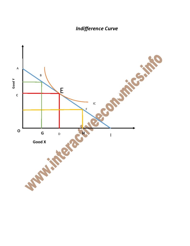
The illustration displays an Indifference curve (IC). The level of customer satisfaction is the same for any combination that lies on this curve. It is also known as the Iso-Utility Curve.

Properties of an Indifference Curve or IC

1) An IC slopes rightward and downward:

This curve represents the fact that when the quantity of one product is increased in combination, the quantity of the other product will decrease. To maintain the same level of satisfaction along an indifference curve, this is crucial.

2) The origin of an IC is always convex:

We can infer from the discussion above that Keeya is becoming less and less willing to part with his clothing as he replaces it with food. The diminishing marginal rate of substitution is demonstrated here. The indifference curve has a convex shape thanks to the rate. There are two extreme cases, though:

 

 i) When two commodities can be used interchangeably, the indifference curve is a straight line with MRS constant.

ii) Two products are the perfectly complement to one another. In a car, an illustration of this would be fuel and water. The IC will be L-shaped and convex to the origin in these circumstances.

3) In contrast to a lower IC, a higher IC indicates a higher level of satisfaction:

 

An increased IC indicates that a consumer favours more products than not.

 

4) An IC doesn’t make contact with the axis:

 

Due to our presumption that consumers consider various combinations of two commodities and desire both of them, this is not possible. In contrast to what we assumed, if the curve touches one of the axes, it indicates that the person is content with just one good and does not need the other.

5) Indifference curves do not cross one another:

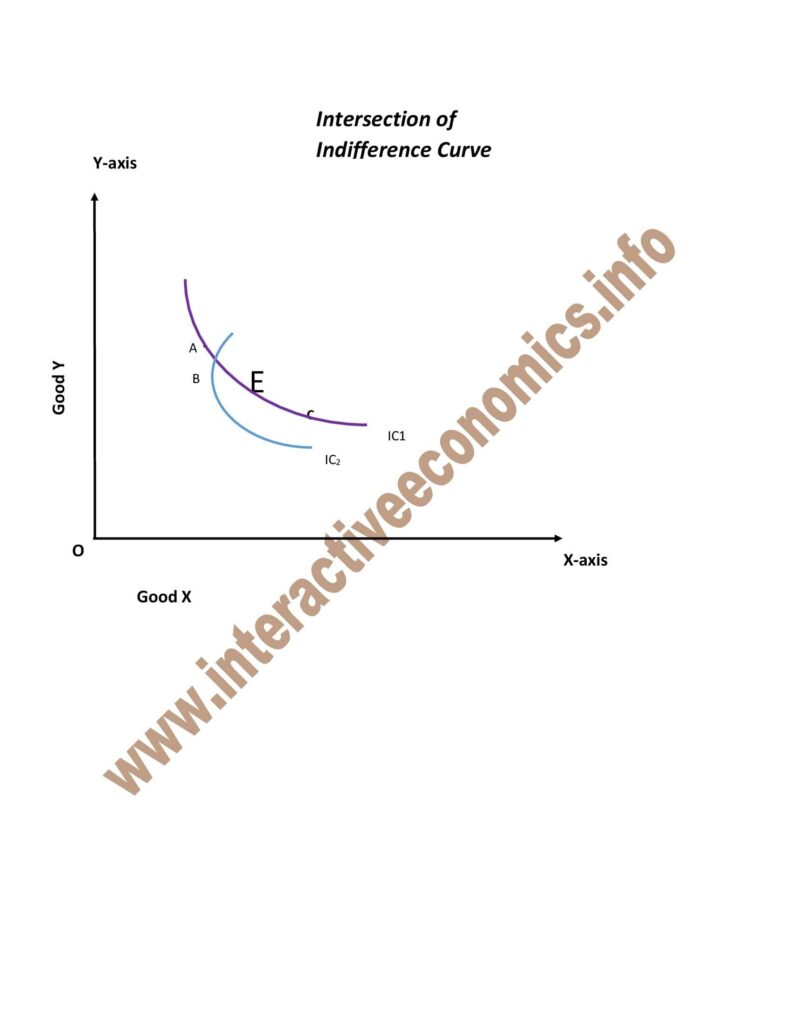
 There will never be an intersection of two ICs. Additionally, they don’t have to run parallel to one another.

Two ICs are shown intersecting at point A in Fig. Points A and B give an individual the same level of satisfaction because they are on IC1. Points A and C, which are also on IC2, provide the same level of satisfaction. As a result, we can infer that B and C provide an equal level of satisfaction, which defies logic. As a result, no two ICs can touch or intersect.

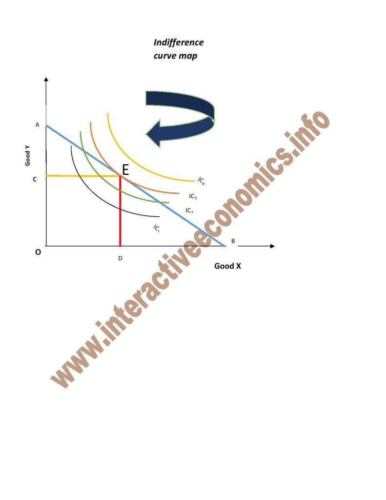
6) The farther out an indifference curve lies, the farther it is from the origin:

An indifference curve’s range increases with distance from the origin and indicates a higher level of utility. The further away from the origin, as shown above on the indifference curve map, the more utility the person produces while consuming.

Criticisms and Complications of the Indifference Curve:

Many aspects of modern economics, including indifference curves, have come under fire for being overly simplistic or making irrational assumptions about how people behave. For instance, consumer preferences may change significantly over time, making accurate indifference curves useless.

 

Others claim that it is theoretically feasible to have circular curves that are convex or concave to the origin at particular points, as well as concave indifference curves. Accurate indifference curves are no longer useful because consumer preferences can shift significantly over time.

The following are some of the main objections to indifference curve analysis:

 

Although there is no doubt that the indifference curve analysis is preferred to the utility analysis, there are many people who disagree. The main criticisms are covered in the section below.

(1) Old Wine in New Bottles:

The indifference cure technique is simply “the old wine in a new bottle,” according to Professor Robertson, who does not discover anything novel about it.

It takes the place of utility with the idea of preference. Introspective ordinalism takes the place of introspective cardinalism. The ordinal numbers I, II, III, etc. are used to represent consumer preferences rather than cardinal numbers like 1, 2, 3, etc. The law of diminishing marginal utility and the principle of diminishing marginal rate of substitution are substituted for marginal utility and marginal rate of substitution, respectively.

The indifference curve technique equates the marginal rate of substitution of one good for another to the price ratio of the two goods, as opposed to Marshall’s proportionality rule or consumer’s equilibrium, which represent the ratio of the marginal utility of a good to its price with that of another good. Thus, this method merely gives the same concepts new names rather than bringing about a positive change in utility analysis.

2) Away from Reality:

Prof. Robertson makes the following comment in response to the claim that the indifference curve technique is better than cardinal utility analysis because it is predicated on fewer assumptions: “The fact that the indifference hypothesis, the more complicated of the two psychologically, happens to be more economical logically, affords no guarantee that it is nearer to the truth.” He goes on to ask if we can disregard four-footed animals that walk on the ground because we only need two feet.

3) Cardinal Measurement implicit in I.C. Technique:

Prof. Robertson adduces that when we examine substitutes and complements, the cardinal measurement of utility is implicit in the indifference hypothesis. In their case, it is deemed likely that the consumer can decide that one change in one circumstance is preferable to another change in another circumstance.

To explain it, Robertson takes three situations A, В and C, as shown in Figure. Suppose the consumer compares one change in situation AB with another change in situation BC.

More so than the change BC, he favours the change AB. He prefers the change AD just as much as the change DC if another point D is taken. Robertson claims that this is equivalent to saying that the space AC is twice the space AD and that we have returned to the world of cardinal utility measurement. As a result, the cardinal measurement of utility is reached when changes in two situations are compared, as in the case of substitutes and complements.

4) Midway House:

Since they cannot be measured directly, indifference curves are purely theoretical. No operational method has yet been developed to precisely determine the shape of an indifference curve, despite the fact that consumer choices are grouped in combinations on the ordinal scale. This results from the theory’s “weird logical structure” and “low empiric content.” Schumpeter labelled the indifference analysis as a “midway house” because Hicks was unable to offer a methodical analysis of consumer behaviour. From a practical standpoint, he observed, “We are not much better off when speaking of purely imaginary utility functions than we are when drawing purely imaginary indifference curves.”

5) Fails to Describe the Consumer’s Observed Behaviour:

Knight contends that there is no objective way to account for the consumer market behaviour that has been observed. It is incorrect to ignore the cardinal utility theory when analysing consumer demand. For example, it is impossible to distinguish between the income and substitution effects based solely on observation. In actuality, the composite price effect is what we see. Comparable to this, the marginal rate of substitution theory of complementaries and substitutes cannot be deduced from market data. In his Revealed Preference Theory, Samuelson explains how consumers act as they do.

6) Indifference Curves are Non-transitive:

W.E. Armstrong is one of the most vocal opponents of the indifference hypothesis. He contends that the consumer is indifferent not because he is fully aware of all the possible combinations, but rather because he lacks the ability to distinguish between them. Additionally, he claims that any two points on an indifference curve are the points of indifference not because they have equal utility but rather because they differ by zero utility.

The relationship between any two or more points on an indifference curve is only symmetrical when utility difference is zero. Figure , where the I1 curve’s points P, Q, R, and S represent various combinations of the goods X and Y, can be used to explain Armstrong’s arguments. The points P and Q, R and S are so drawn that the difference between each pair is imperceptible.

Points P and Q or R and S won’t have equal utility unless there is no utility difference between them. However, the consumer cannot be neutral between P and R because there is a discernible difference in the total utility between the two. Thus, the consumer will choose P over R, or R over P in the opposite situation. This demonstrates that an indifference curve’s points are not transitive. According to Armstrong, “the textbook diagrams with their masses of non-intersecting indifference curves do not make sense if indifference is not transitive.” Thus, the very idea of “indifference” seems to have questionable validity.

(7) The Consumer is not Rational:

The utility theory and the indifference analysis both presuppose that consumers behave rationally. He has a calculative mind, can substitute one good for another, compares the total utilities of different combinations of goods, and can make logical decisions when faced with a variety of options. It is unreasonable to demand this of consumers who are subject to a number of social, economic, and legal restrictions.

(8) No principle is used to base combinations:

The combinations are made regardless of the nature of the goods, so they frequently turn absurd. How many of us would buy six radios and five watches, four scooters and three cars, or ten pairs of shoes and eight pairs of pants? For the consumer, these combinations are meaningless.

(9) Limited Analysis of Consumer’s Behaviour:

Furthermore, it is unjustified to assume that when a product’s price drops, consumers will purchase more of the same item. Aside from the situation where the product is subpar, he might not want more than one unit of a product because he practises “conspicuous consumption” and wants to show off or have variety. The consumer’s preference for the goods is also influenced by changes in his tastes or by speculative purchases. The indifference analysis is a constrained examination of consumer behaviour because of these exceptions.

(10) Failing to take into account some other variables affecting consumer behaviour:

The Veblen and Bandwagon effects, the effects of advertising, the effects of stocks, etc. are not taken into account by the indifference curve analysis. Neither are speculative demand, the interdependence of consumer preferences in the form of snobs, or speculative supply.

(11) Two-Goods Model Unrealistic:

Once more, the two-goods model, upon which the indifference analysis is based, renders the theory implausible because a consumer purchases many more goods than just two in order to satisfy all of his numerous desires. But the problem is that geometry breaks down when there are more than three goods, forcing economists to rely on challenging mathematical formulas to analyse the issue of consumer behaviour.

(12) Failing to Describe Consumer Behaviour When Making Risky or Uncertain Decisions:

The preference hypothesis has also come under fire for failing to explain how consumers behave when given choices that involve risk or unpredictability of outcomes. If there are three possible outcomes—A,, and C—the consumer prefers A to and C to A, with the knowledge that A is guaranteed but that either or has a 50/50 chance of happening. The consumer’s preference for over A in this instance can only be quantified.

(13) Based on Unrealistic Perfect Competition Assumption:

The indifference curve technique is based on the unrealistic assumptions of perfect competition and homogeneity of goods when, in fact, consumers must deal with differentiated products and monopolistic competition. The indifference hypothesis loses credibility because it is founded on erroneous presumptions.

(14) Not all commodities can be divided:

When it is assumed that goods can be divided into small units, the indifference curve analysis looks ridiculous. Things like watches, cars, radios, and other commodities cannot be divided. It is unrealistic to have 3½ watches, 2½  cars, or 1½  radios in any combination. Indivisible goods cannot be substituted in a combination without first being divided. Therefore, the consumer cannot use indivisible goods to their fullest potential.

Despite these objections, the Marshallian introspective cardinalism is still thought to be inferior to the indifference curve method.

Limitations of Indifference Curve:

Because it is more accurate, indifference curve analysis is said to be superior to utility analysis. But because it is based on some irrational assumptions, it continues to draw criticism from many economists. Additionally, according to Schumpeter, “The new technique has neither proved anything new, nor has it proven anything old, wrong.”

This analysis was blamed by Robertson, who described it as “old wine in a new bottle.” Numerous other economists, including F.H. Knight, Armstrong, and Boulding, offered numerous criticisms of the analysis. The following are a few of this analysis’ limitations:

1. The utility analysis in a new grab is the indifference curve analysis. It has merely used new equations and concepts in place of the outdated ones. The new principle of diminishing marginal rate of substitution has taken the place of the previous principle of diminishing marginal utility. the dated consumer equilibrium equation.
2. A new equation that states that the consumer is in equilibrium when the marginal rate of substitution between the two commodities, which is the ratio of their marginal utilities to their price ratio, replaces MUA/PA = MUB/PB = MUM. This is nothing more than a modified version of the previous equation.
3. The analysis of the indifference curve makes the assumption that consumers are aware of their preference schedules. The total satisfaction from all possible combinations of the two commodities, as well as the rates of substitution and total incomes, cannot be known by a consumer. He can only give his preferences in the general area of his current position. Furthermore, this consumer’s preferences are ever-evolving.

4. Only two commodities are included in this analysis. It is necessary to treat one commodity, let’s say ‘Y,’ as a composite commodity (represented by money) in order to cover a large number of commodities, so that the prices of all the commodities that make up the composite commodity change simultaneously and proportionately.

This might not actually occur. Separating the impact of a change in a specific commodity’s price also gets challenging. Although it is challenging to handle, we can also use a three-dimensional diagram for the case of three goods. When it comes to handling situations with more than three goods, geometry completely fails. In such a case, we might have to resort to challenging algebraic techniques.

5.The analysis makes the assumption that consumers are rational. However, consumers frequently act in an irrational and callous manner.

6. Indifference curve analysis is introspective because it examines consumer behaviour using fictitious indifference curves that are drawn. Additionally, it is founded on a flimsy ordering hypothesis. Consumers are therefore uninterested in certain combinations. This analysis was criticised by Samuelson because when a customer selects a certain combination, he favours it over all other combinations. As a result, “choice reveals preference.” Samuelson developed the more scientific demand theory based on observed consumer behaviour.

7. This analysis presupposes that the commodities are completely divisible. But lumpy units are a common problem for consumers. Therefore, despite the fact that there are many indifference curves that are placed very close together, the continuity of indifference curves is not guaranteed as claimed by indifference curve analysis. Additionally, extreme combinations (too much of a given commodity X and very little of a different one Y, or vice versa) are not seen in the real world.

8. The microeconomic nature of the analysis of the preference curve. Drawing indifference curves that represent a group’s or a nation’s overall preferences is not possible. Utility analysis has an advantage in this regard because it bases its conclusions on an overall assessment based on prior experience and observation.

9. Because the entire analysis is based on theoretically formulated cross-effect relationships rather than statistical observations, indifference curve analysis is not amenable to statistical investigation and empirical research. Samuelsson believes that indifference curves are hypothetical.

10. The analysis of the preference curve is unable to account for consumer behaviour in risky and uncertain situations.

As a result, indifference curve analysis has flaws of its own. Hicks acknowledged some of these flaws and attempted to fix them in his 1956 publication, “A Revision of Demand Theory.” The method has become more and more popular among economists because it is a significant improvement over the traditional utility approach.

Derivation of demand curve under indifference curve approach:

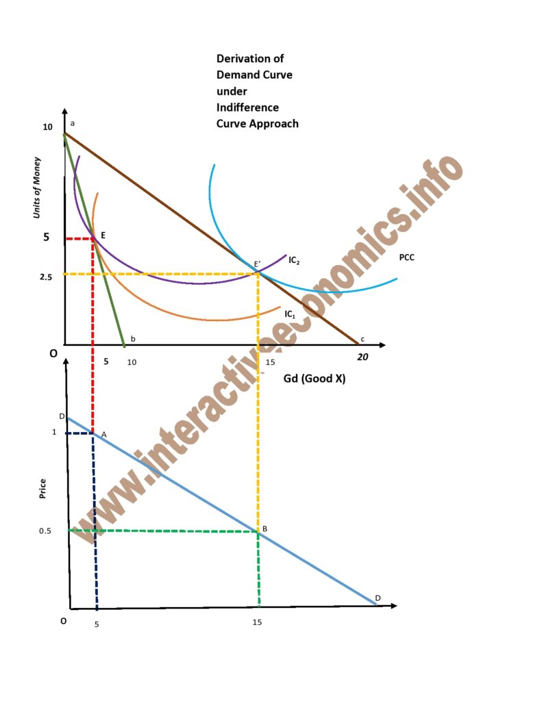
Following are two diagrams explain from/with the derivation of demand curve under the indifference curve technique. The income of the consumer is fixed at Rs. 10/-.

 In the top figure, on the horizontal axis is the Q_d of good X and the vertical axis are the purchase 5 units of good X. It will cost him Rs. 5/- and will leave him with a balance of Rs.5 price of good X goes down to Rs. 0.50/-.

The consumer still has the same income of Rs. 10/- but his budget line will be at ac because he is able to purchase more of good X. Here he decides to purchase more of good X and this will cost him Rs. 7.5/- leaving with him Rs. 2.5/-.Thus his new equilibrium point has shifted from E to E’. Bottom figure is just to explain the units of good X purchased by the consumer at different price. Hence 5 units at Rupee 1 per unit and 15 units at Rs. 0.50/- per units are purchased. Combining the two points A and B, we get the demand curve DD.