Consumer’s Equilibrium
January 2, 2023
The consumer’s equilibrium is a situation in which a consumer spends his given money on one or more commodities to maximise pleasure and has no desire to modify this level of consumption, given commodity prices.
The phrase equilibrium refers to a condition of rest in which there is no propensity for anything to change. A consumer is said to be in equilibrium when he or she does not want to adjust his or her level of consumption, i.e. when he or she achieves maximum satisfaction. As a result, consumer equilibrium refers to the condition in which the consumer has obtained the most potential pleasure from the quantity of goods purchased given his/her income and the price of the product.
When a consumer thinks that he cannot improve his circumstances by earning more, spending more, or increasing the amount of products he purchases, he is said to be in an equilibrium state. A rational buyer will buy a product until the price of the item equals the marginal utility derived from the object.
If this criterion is not met, the consumer will either buy more or buy less. If he buys more, the MU will decline, and there will be times when the price paid will surpass the marginal utility. To avoid negative utility, or discontent, he will cut his consumption, and MU will continue to rise until price equals marginal utility.
Consider the basic situation of a buyer who is only interested in consuming two goods: good One and good two. This consumer is aware of the pricing of products one and two and has a set income or budget from which to acquire quantities of commodities One and two. The buyer will buy enough of commodities one and two to entirely deplete the budget for such purchases. According to this criterion, the marginal value per dollar spent on good one must match the marginal utility per dollar spent on good two. If, for example, the marginal utility per dollar spent on good one is greater than the marginal utility per dollar spent on good two, the consumer would be wise to buy more of good one rather than any more of good two. As more of good One is purchased, its marginal utility will eventually reduce according to the rule of declining marginal utility, such that the marginal utility per dollar spent on good one will finally equal that of good two. Of course, the quantity spent on commodities one and two cannot be infinite and will be determined not only by the marginal utility per dollar spent, but also by the consumer’s budget.
In the Case of a Single Commodity, Assumptions for Achieving Consumer Equilibrium
Assume the following for a single commodity:
1) The purchase would be limited to a single commodity.
2) The commodity’s price is already set in the market. The consumer just decides how much he needs to buy at a certain price.
3) A consumer’s purpose, as a rational human being, is to maximise his consumer surplus, which is the surplus of utility he obtains over his expenditures on the commodity at the moment of purchase.
4) There are no restrictions on consumer spending, which means he has enough money to buy whatever amount he wants at a given price.
In the Case of Two or More Commodities, Assumptions for Achieving Consumer Equilibrium
Assume, in the case of two or more commodities:
1) The buyer buys only two products, i.e. A and B.
2) The market price for both commodities is already known. The pricing of both commodities cannot be changed or influenced by the consumer. He can only determine how much of these products to purchase at a particular price.
3) The consumer’s income to spend on these things is predetermined and consistent.
4) The consumer is a rational human being whose purpose is to maximise the (cardinal) quantity of utility from the products he purchases and consumes within his limits.
Consumer Equilibrium in the Case of a Single Commodity
The consumer equilibrium may be explained using the law of diminishing marginal utility in the case of a single commodity. According to the law of declining marginal utility, when consumers consume more and more units of goods, the marginal utility obtained from each succeeding unit decreases. As a result, how buyers select how much to buy is determined by the two elements listed below.
1) He/she is provided the price for each product purchased.
2) The utility he or she receives
A consumer compares the price of a product with its utility when acquiring a unit of that product.
A consumer compares the price of a product with its utility when acquiring a unit of that product. When the consumer’s marginal utility (in terms of money) equals the price paid for the product, say ‘X,’ he or she has reached an equilibrium state.
MUx = Px
If MUx exceeds Px,
When MUx exceeds price, the consumer continues to buy the product since she is paying less for each increased level of satisfaction he is receiving. As she purchases more, MU falls, and instances emerge in which the price paid exceeds marginal value ( the concept of the law of diminishing marginal utility is applied here). To prevent this circumstance, he will reduce his intake, and MU will continue to increase until MUx = Px. This is the equilibrium state.
If MUx less than Px,
When MUx is less than price, the consumer must reduce his usage of the product in order to increase his overall pleasure until MU equals price. This is due to the fact that she is paying more than she is receiving in terms of added satisfaction.
Consumer Equilibrium in the Case of Two or More Commodities:
In the case of two or more goods, the law of declining marginal utility does not apply. In most cases, a consumer will consume more than one commodity. In such a case, the rule of equity-marginal utility is employed to assist him in determining the best distribution of his income. According to the law of equi-marginal utility, a consumer should spend his limited money on various goods in such a manner that the last rupee spent on each product gives him with equal marginal utility in order to achieve maximum satisfaction.
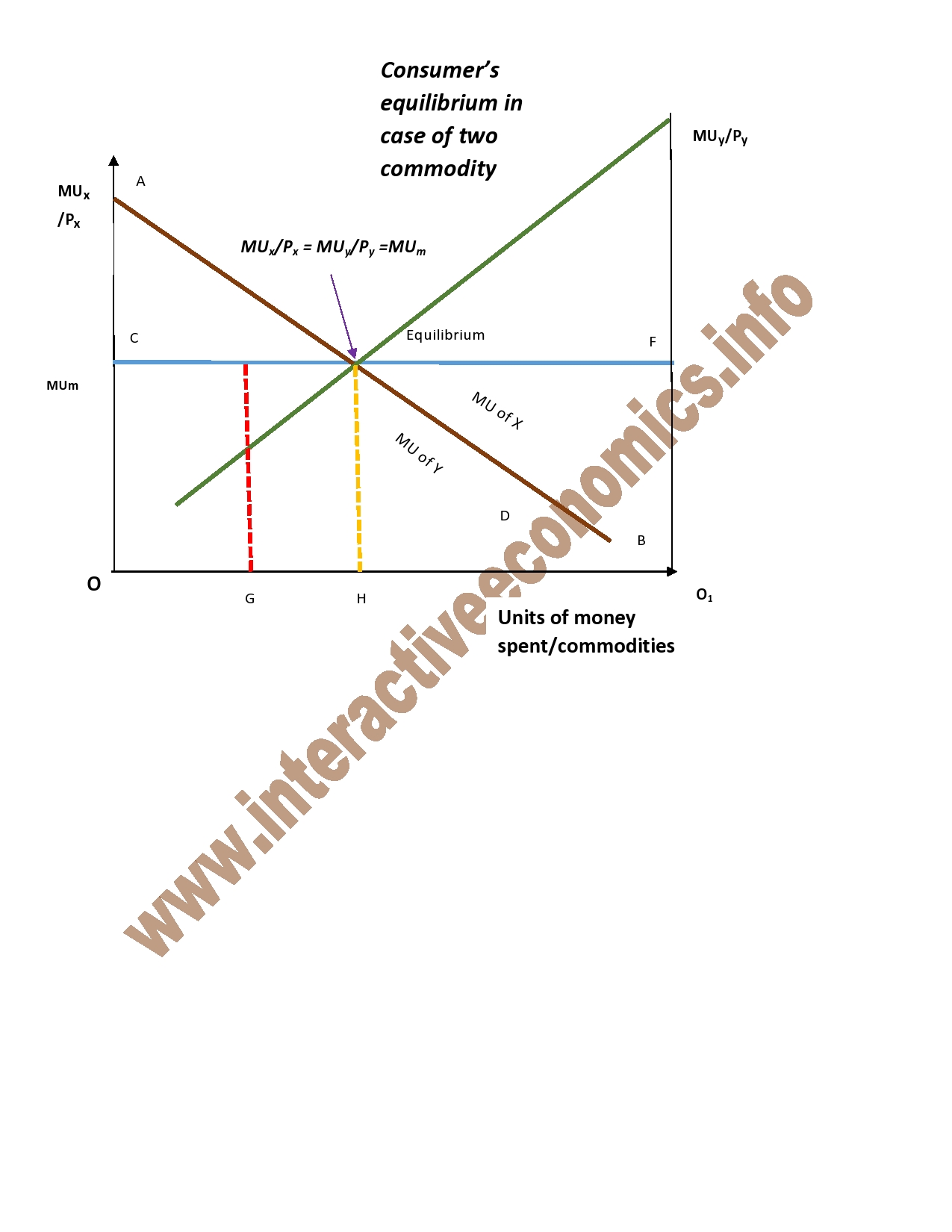
A consumer will be in equilibrium when the ratio of marginal utility of one commodity to its price equals the ratio of marginal utility of another commodity to its price, according to the law of equi-marginal utility.
Assume that buyers purchase two products, X and Y. The equilibrium pricing stage will then be at
MUx/Px = MUY/PY = MU of the most recent rupee spent on each commodity, or simply MU of Money.
Likewise, if there are three commodities, namely X, Y, and Z, the condition of equilibrium will be simply MY Money.
To achieve an equilibrium position,
1. The final rupee spent on each commodity has the same marginal utility.
2. A commodity’s marginal utility decreases as more of it is used.
Consumer’s Equilibrium by Indifference Curve Approach
We know that a consumer is indifferent among indifference curve combinations. It is worth noting, however, that they favour combinations on the higher indifference curves to those on the lower ones. This is due to the fact that a greater indifference curve indicates a higher level of satisfaction. As a result, all combinations on IC1 provide the same level of satisfaction, whereas all combinations on IC2 provide higher levels of satisfaction than those on IC1. To find the equilibrium point, the consumers evaluate the price (or cost) of a specific product against its utility (satisfaction or benefit). They will be in equilibrium as a rational consumer when the price paid for the product equals the marginal utility. Price and marginal utility are both expressed in terms of utils. However, marginal utility and price can only be compared when stated in the same units. As a result, utils’ marginal value is expressed in monetary terms. Money-based marginal utility = utils/M marginal utility. Similarly, if three goods are present, X, Y, and Z, the equilibrium condition is simply MU Money. As a result, to be in equilibrium
1. The marginal utility of the last rupee spent on each product is the same.
2. A good’s marginal utility decreases as more of it is consumed.
Assumptions
1) There is a specified indifference map displaying the consumer’s preference scale across various combinations of two commodities X and Y.
2) The consumer has a set amount of money and want to spend it entirely on the commodities X and Y.
3) The consumer’s pricing for the commodities X and Y are fixed.
4) The commodities are uniform and divisible.
5) The buyer behaves logically and seeks maximum satisfaction.
6) The consumer’s income is fixed.
7) The two income-purchased commodities can be replaced for one another.
8) The sensible client strives to maximise their level of satisfaction at all times.
9) The price of things is fixed.
10) The consumer is aware of the commodity pricing.
11) Consumers can spend their money in modest amounts.
12) The market is fiercely perfect competition.
13) The products are divisible.
14) The consumer is familiar with the indifference map.
Consumer’s Equilibrium under various situation:
1.Under Income Effect :
A change in the income of a consumer will result in a change in consumer’s equilibrium. The effect of income on the consumer’s equilibrium can be divided into two parts.
- Income effect when both goods are Normal Goods:
With a rise in income, two products that are normal goods are purchased more by the consumer. Normal goods here simply refers to any type of the commodity with neither of its impact on the consumer.
This is the diagram explaining the income effect on the consumer’s equilibrium.
When the budget line is ab, IC1 is the curve and the consumer is in equilibrium at point E with the given income. There, he makes a combination of ON amount of good X and OM amount of good Y. When his income increases, his budget line moves in a parallel manner. Hence, he is at IC2 and his equilibrium point is E1 which also shift in the same manner from E. There he purchases more of both goods as they are normal goods. Thus ON amount of good X and OM1 amount of good Y are purchased.
Again as his income rises, he will move to the IC3 budget line of ef and equilibrium point of E2. Thus more of both goods, i.e. ON2 of X and OM2 of Y are purchased. Therefore, by joining points E,E1 and E2 together to the origin, we get a curve known as the income consumption curve ICC, which explains us that with each addition to the income of a consumer, he will purchase more of both the normal goods and vice versa.
(b) Situation when there exists a superior and inferior goods:
When one product is superior and the other is inferior, he will purchase more of the superior good and less of the inferior good. Superior here refers to any goods which is of more use or is needed more by the consumer than the other good.
From the basic equilibrium point E, the consumer purchases ON amount of Good X and OM amount of good Y. With an increase in his income, his budget line moves from ab to cd. Thus, this equilibrium points also shifts to E1 where the new budget line makes a tangent which is IC2. Here he purchases ON1 amount of good X and OM1 amount of good Y. Similarly, with a change of equilibrium point of E1 to E2 , his income increases. Thus, creating a new budget line i.e. ef and he purchases ON2 amount of good X and OM2 amount of good Y.
From the diagram, we clearly see that he purchases more of good X, i.e. superior good and less of good Y i.e. inferior good as his income increases. Therefore, by joining points E, E1 and E2 together. It is clearly seen the ICC is bending towards the horizontal axis, i.e. superior good, stating that the consumer is purchasing more from this axis.
(b.1) Income effect when Y is a superior good and X is the inferior good:
At the basic equilibrium point E, the consumer’s budget line is ab. At this point, he purchases OS amount of good X and OM amount of good Y.As his income increases his budget line also shifts to cd and he reaches at Equilibrium point E1. As his income increases again, it results in another shift of his budget line i.e. from cd to ef. And
With this budget line, he achieves equilibrium point E2 where he purchases OU amount of good X and OQ amount of good Y. From this diagram, we are able to make out the fact that the consumer purchases more of good Y and less of good X as his income increases. This proves that Y good is the superior good and X good is the inferior good.
2. Price effect on Consumer’s Equilibrium:
(i) With the fall of the price of good X:
This diagram explains the effect on the consumer’s equilibrium when the price of good X falls. The income remains fixed. At the basic equilibrium point E, the consumer purchases OZ amount of good X and ON amount of good Y. As the price of good X falls down, the purchasing power of the consumer seems to have changed, however, not really. This only means that the consumer has more money to spend on a certain good i.e. good X as its price has gone down. We find that the consumer’s equilibrium shift to E1, he purchases OI of X and OM of Y on IC2.As the price of good X falls down again the consumer purchases more the cheaper good and less of the dearer one. Hence, there is a change in equilibrium point to E2.Here he purchases OB of X and ON of Y on IC3. This diagram shows that PCC is bending towards the horizontal axis indicating that consumer purchases more of a cheaper product and less of the other which now seems dearer.
(ii) With the fall of the price of good Y:
At point E on IC1, the consumer purchases ON of good X and OQ of good Y.As the price of good Y decreases, the consumer is tempted to purchase more of good Therefore, at point E1 on IC2, he purchases of OM of good X and OR of good Y, hence an increase of good Y. As the price of good Y decreases further, good X seems to be dearer to the consumer. Therefore, he purchases more of good Y and less of good X. This is shown in the equilibrium point of E2 on IC3 where the consumer purchases OL of good X and OS of good .Here, income of the consumer remains constant. The PCC is bending towards the vertical axis showing that the consumer goes for the cheaper product, i.e. good Y.
3. Substitution effect:
In this diagram initial equilibrium is at point E on IC1. When the price of good X falls the budget/price lines move from ed to ef and the new equilibrium point is attained at E’ on IC2. With the fall in the price of good X, consumer’s real income increases. Therefore, to keep its real income constant, we reduce consumer’s money by shifting budget line at E”. Thus the movement from point E to E” on IC1 represents the Substitution effect of the price change. According to which the consumer substitutes NH of good Y with MK of good X.
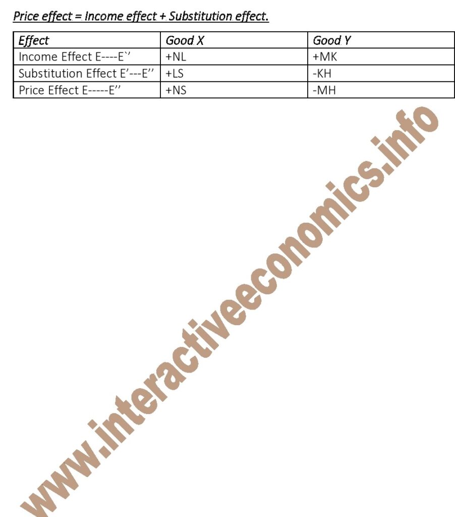
Price Effect = Income effect + Substitution effect :
Modern economists have made out it is the price effect which brings all the changes. The diagram above kills three birds with one stone. We are combining together the price, income and substitution effect.
At the basic equilibrium point E on IC1, the consumer purchases ON of good X and OM of good Y. In the case, both goods are normal goods. With the change in income (i.e. his income increases).The new equilibrium point is E’ on IC2 where he purchases OL of good X and OK of good Suppose the price of good X good goes down, due to the low price of good X, the consumer’s tendency to purchase more of it arises. Therefore, he makes a substitution for it. He purchases KH less amount of good Y for LS of good Hence his new equilibrium point is E” on IC2.Thus, we are able to make a triangle showing price effect, income effect and substitution effect, according to which Price effect = Income effect + Substitution effect over Substitution.
Ordinary inferior good:
Our explanation is mainly on the inferior good .The consumer encounters a negative income effect on the inferior good X, i.e. Q1Q2. Since his income increases. Therefore, he is on IC2 and his new equilibrium is E”.
In the market, the price of the inferior good X decreases. However, this consumer cannot shift to a new budget line or price line as his income is still the same. Therefore, an imaginary budget line, i.e. ae is made so that the IC2 touches the line where the consumer makes a substitution effect Q2 Q3 is positive for good Since positive substitution effect is greater than the negative income effect, hence here is a positive price effect on good This shows that good X is an ordinary inferior good.

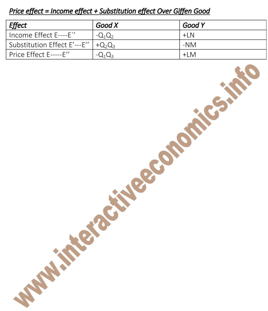
Giffen good:
When the income on the consumer increases, his equilibrium shifts from E to E’. In conjunction with this, the price of inferior good X decreases. However, substitution made weaker than the negative income effect. Since, negative income effect is greater than positive substitution effect, thus, price effect is negative i.e. Q1Q2 on the inferior good. Hence, good X is a special kind of inferior good called Giffen good.