When we consume a thing, we are expressing our desire for it. As a result, there must be a market supply for it. Clearly, we want to pay the lowest price possible for what we desire, while the seller wants to extract the greatest price possible from us in order to maximise his profit. The equilibrium price is determined by the point at which the quantity demanded is exactly equal to the quantity supplied. Therefore, price is determined by the Equilibrium of demand and supply or by the free play of the forces of demand and supply under perfect competition.

Explanation with Table and Diagram:

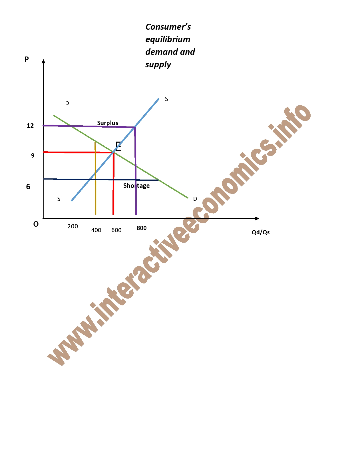
We can see that Qd= Qs at 600 kg where the price is Rs. 9. Therefore, the equilibrium price is Rs. 9 and 600 kg is the equilibrium quantity.

The above table can be converted into a diagram as given:

From the diagram we can see that where the curves intersect each other, the equilibrium price and quantity are demanded. Hence, at price Rs. 9 equilibrium quantity is 600 kg. Any change would not benefit either the consumer or seller. For example, if the price goes up to Rs. 12, Qd is 400 but Qs is 800 thus price decreases to Rs. 9. If the price decreases to Rs.6, Qd is 800 but Qs is 400. Therefore, in order to reach an equilibrium, the price must be set at Rs. 9.

Effects of changes in demand and supply:

Effects of changes in demand:

Basic equilibrium point E. With a rise in demand, Qd/Qs increases to OQ’ price also rises to OP’. With a fall in demand Qd/Qs goes down to OQ’’ and price also decreases to OP’’. Hence, this is the effect of a rise and fall of demand.

Effects of changes in supply:

Basic equilibrium point E. Fall in supply brings Qd/Qs to OQ’ and leads to a rise in price to OP’. Rise in supply up to OQ’’ leads to fall in price to OP’’.

Effects of changes in both demand and supply:

Basic equilibrium is at E where price is OP and quantity is OQ. With a rise in demand and fall of supply more proportionality E’ becomes the new equilibrium point. Thus price rises to OP’ and quantity falls to OQ’.

Important of Time Element in the determination of Price:

The time element can be sub-divided into three categories:

• Very short period
• Short period
• Long period

All these three periods are related to supply e.g. (i) is also known as the market period where the supply is fixed, as the goods have to be disposed of as quickly as possible. For example, agricultural products. In (ii) some of the factors of production are fixed, such as machinery/plant and land etc. Whereas others, such as labour and raw material are variable. They can be increases or decreased in accordance with the will of producer. The products in this time period can be stored up if there is not much demand for them. E.g. .Stationery etc. Here elasticity of supply is less than unity whereas in very short period products, elasticity of supply (e.o.s) = o.i.e, supply is perfectly inelastic. (iii) Examples of long period products are refrigerator, T.V’s etc. They can also kept in stock. Their supply varies and here e.o.s. is more than unity because all factors of production are variables (i.e. all the four factors can be increased to get more products).

Determination of market price:

Therefore, the equilibrium price is Rs. 20 for equilibrium price is Rs. 20 for equilibrium quantity of 40kg.

Here is the diagram for perishable goods at the market price. These goods have to be disposed of quickly. Therefore, as we see above, the supply is fixed and demand plays the dominant role. With a rise in demand, as we see at E’, the price goes up to Rs. 24. And with a fall in demand, the price also decreases to Rs. 16 as seen at the equilibrium point E’’.

Therefore, we can conclude that the market price of perishable goods depends very much on the demand for them as they have to be disposed of quickly as possible, and at the same time seller wants to gain maximum profit, therefore, the price is quite flexible!

Market Price of durable commodities:

Therefore, equilibrium price is Rs. 20 for equilibrium quantity of 25 pens. The above diagram shows the effect of change in demand on the price of durable commodities in the market.

The supply of pens is fixed at 30 although it can be initially increased by taking more out of the stock. Basic equilibrium point E with equilibrium price being Rs. 20 for 25 pens. With a rise in demand price changes slightly to Rs.25 shown by equilibrium point E’. However, as the demand for pens still increases; this will shoot the price up to Rs.40 as its supply is limited for that particular day. Again demand plays a dominant role in fixing the price.

Market price and normal price:

• In case of very short products, demand for it dominates the whole situation of price. Supply is fixed as the products must be disposed of as quickly as possible. Therefore, price matches demand. This is known as market price.
• The price of short and long period products is known as the normal price. This is because price for these products is determined through the interaction of both demand and supply.

Normal price of short period products:

In this case supply of products is inelastic and e.o.s < unity. From the diagram, the basic equilibrium point is E. Therefore, price is equal to EQ and the quantity supplied is OQ. With a rise in demand, i.e. to D’D’ the quantity supplied only changes slightly i.e. to OQ’ whereas the change in price is quite sharp i.e. from EQ to E’Q’. With an adequate fall in demand to D’’D’’, supply again changes slightly i.e. to OQ’’ but the price decreases quite sharply i.e. from EQ to E’’Q’’. Therefore, we can see that even with an applicable change in price there is only a slight change in supply.

Normal price of long period products:

Examples of long period products are refrigerators, radios, televisions etc. Supply of these products is said to be elastic as price effect on these products causes an adequate change in supply and demand. Basic equilibrium point is E, price is EQ and supply and demand is OQ. With a small increase in price i.e. EQ to E’Q’, we can see that quantity demanded and supplied has risen adequately. Similarly, when the price decreases i.e. EQ to E’’Q’’ quantity demanded and supplied respectively fall adequate to OQ’’. Therefore, in case of long period products they prove to be elastic.

Comparison of the time periods with rise and fall of demand:

Following is the case for a rise in demand and the different effects in the three time periods. Basic equilibrium point is E, quantity supplied here is OS. In the market period, the supply is fixed and is perfectly inelastic. Therefore, as the demand goes up for their product as shown by D’D’ the price in the market period shoots up to PS. In short period, supply is not fixed and is inelastic. Therefore, as we can see an adequate change in supply i.e. to OS’, the price slightly moves to S’S’. In long period, the supply is elastic, therefore, with a big change in supply as shown by OS’’ due to the rise in demand, the price for these products only changes a little bit.

Following is the case for a fall in demand and its effect in various time periods. In the market period, supply is fixed, therefore, with a fall in demand, price falls sharply. In the short period, supply is inelastic and with a fall in demand, there is also a slight decrease in supply i.e. to OS’. Therefore, the price decreases only a little bit. In the long period, supply is elastic. So with a fall in demand, there is a great contraction in supply i.e. to OS’’ and only a small drop in price.